The First Thousand PSFs

In my last post on my PSF Project I characterized the PSF shape by fitting a 1-D Gaussian to the a row and column slice through the central pixel. In this post I start to think about how to characterize entire images with thousands of stars.

Adding Some Zeros

Many applications for the PSF database involve looking at PSF changes over a time series. One way to do this is to move from characterizing individual PSFs to characterizing the PSFs in an entire image and seeing how that changes over time. ¹ In other words, we need to add some zeros to our lone star and start working our way towards our final dataset of 10 million. I decided to do this by digging into the first stellar field I could find. This happened to be iabj01a2q_flt.fits an image of NGC104 which adds 3 more zeros to our star total, bringing it to roughly 1,500 stars. Here is the image, it's actually quite nice (sorry for the large file):

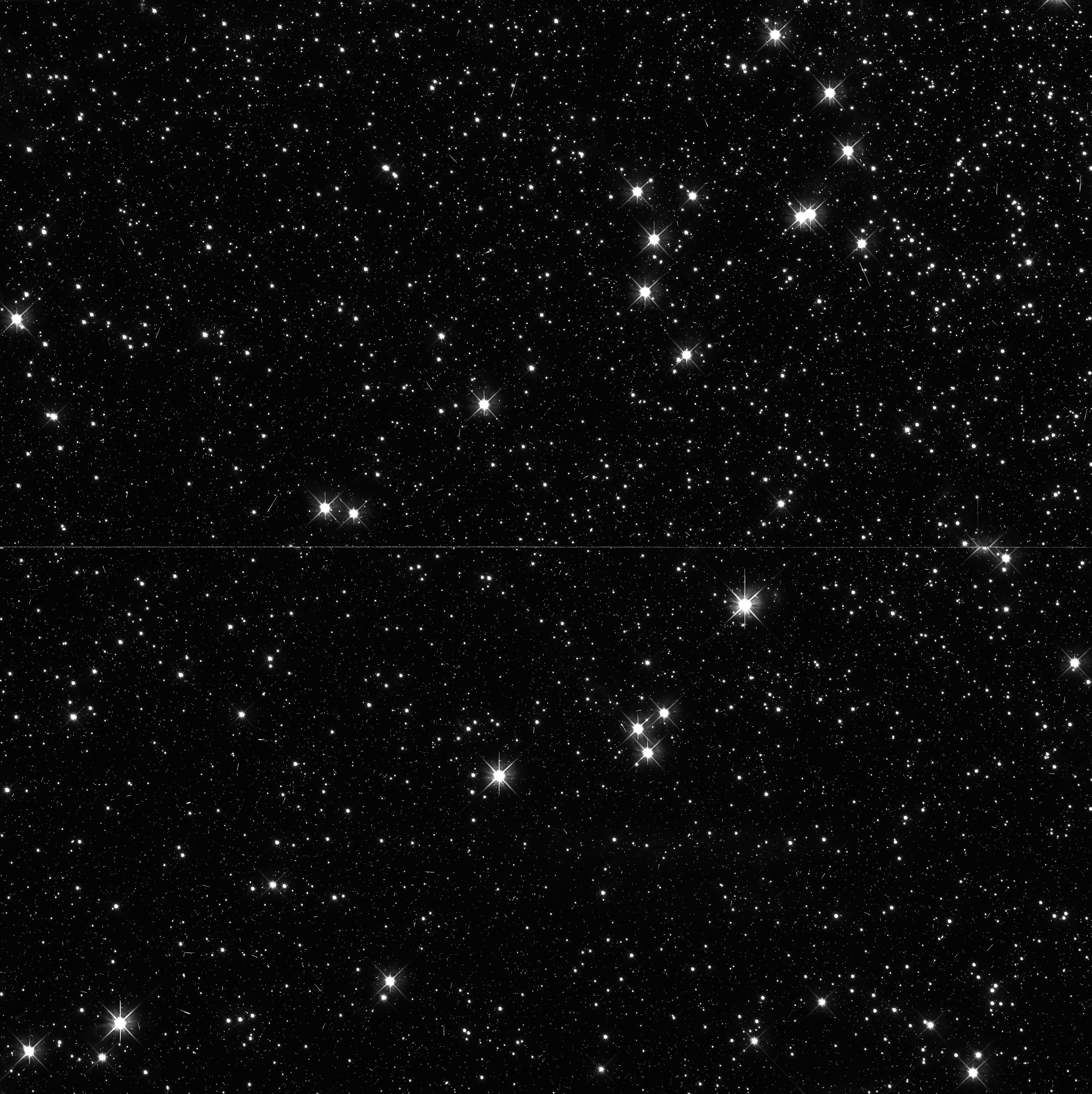
In case you want to play along at home, this image is in the public domain and can be found here.

Plotting the PSF Fits

So I went ahead and fitted a Gaussian in both the row and column directions for all the stars in that image. Then I studied the distribution by plotting the fit parameters against each other in each slice.

First of all, in hindsight what I wanted was a scatter plot matrix but this is exploratory work so I can go back and make that plot in the future.

In terms of the actual data, we don't see anything noticeably different between the row and column slices, which is expected at this point, though there there may be directionally-dependent instrumental effects, such as the charge transfer efficiency, which may come into play later. Looking at the individual fit parameters there's not much going on with the amplitude but things get interesting when we plot the standard deviation against the mean (mu). However, the correlation we're seeing in the plot is actually a sampling effect.

Interpreting the Results

Let's start by explaining what sigma and mu mean in this context (it might be helpful to refer to my last post). First of all, mu, the mean of the Gaussian fit is almost always between 4.5 and 5.5. This is by design because the algorithm that centers the PSF cutouts does a good job of picking the brightest pixel. sigma then is a measure of the width of the PSF.

The actual energy distribution of a star is a continuous distribution. However, detectors take discrete samples from this distribution, pretty much literally making a histogram. If you've played around with histograms much you might see where this is going. If a star happens to land exactly in the middle of a pixel (mu = 5) most of the light from the PSF will land in that pixel. This will result in a narrow sigma. But is the same PSF lands right in the middle of two pixels (equidistant from their centers) then the same amount of flux is split between those two pixels. The total amount of flux is still the same, but the distribution is different. This distribution is less peaked, which is to say wider and with a larger sigma.

I think this is supported by the fact that as you move away from the middle of the central pixel (mu = 5) the distribution of sigma for a given mean moves up (gets wider) in an absolute sense, but not in a relative sense. Put another way, the width of you PSF increases the further the peak is from the central pixel, but the difference between a peaked and broad PSF at any given mean is about the same.

What's Next?

The next step is pretty clear, we need to use this distribution of parameters to characterize the "average" PSF shape in each image and plot that as a time series. This will almost certainly yield nothing but noise, but I'm confident that as we tease the data out such as separating each filter or different parts of the detector we'll start to see some real trends.

But, this sampling effect is bothering me. If we just take a mean and standard distribution of all the sigma parameters in each image those results are going to be heavily influenced by the sampling effect (I'm deliberately trying to avoid saying the sigma of the sigmas.). However, after looking at a sample set of plots I think this is likely characteristic of all our data. Consistency will have to suffice for now because as you'll see in my next post there are more pressing problems as we start to add zeros to our star count.